Robots

Coordinate frames

One of the most basic concepts related to robotics that COMPAS provides are coordinate frames, which are described using the compas.geometry.Frame class.

In any robotic setup, there exist multiple coordinate frames, and each one is defined in relation to the next. Examples of typical coordinate frames are:

• World coordinate frame (WCF)

• Robot coordinate frame (RCF)

• Tool0 coordinate frame (T0CF)

• Tool coordinate frame (TCF)

• Object coordinate frame (OCF)

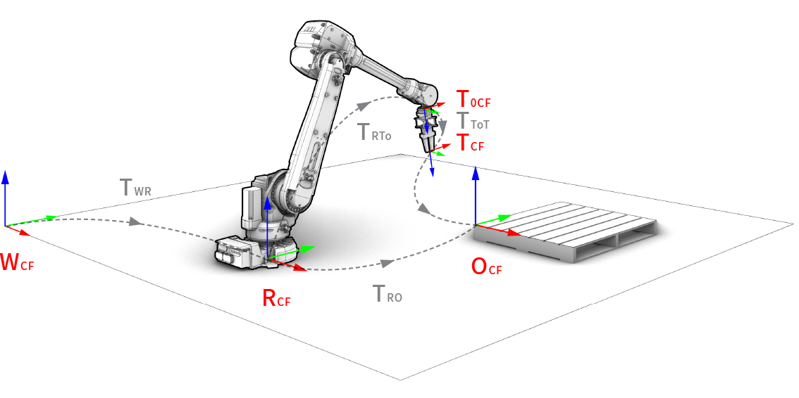
Coordinate frame convention of a robotic setup.

A coordinate frame is defined as a point and two orthonormal base vectors (xaxis, yaxis). Both the point and the vectors can be defined using simple lists of XYZ components or using classes. Frames are right-handed coordinate systems. The following two examples are equivalent:

>>> from compas.geometry import Frame, Point, Vector

>>> frame = Frame([0, 0, 0], [1, 0, 0], [0, 1, 0])
>>> frame.point
Point(0.000, 0.000, 0.000)

>>> frame = Frame(Point(0, 0, 0), Vector(1, 0, 0), Vector(0, 1, 0))
>>> frame.point
Point(0.000, 0.000, 0.000)

There are shorthand constructors for the frames located at (0.0, 0.0, 0.0):

>>> f1 = Frame.worldXY()
>>> f2 = Frame.worldYZ()
>>> f3 = Frame.worldZX()

And there are additional constructors to create coordinate frames from alternative representations such as:

>>> f4 = Frame.from_axis_angle_vector([0, 0, 0], point=[0, 0, 0])
>>> f5 = Frame.from_points([0, 0, 0], [1, 0, 0], [0, 1, 0])
>>> f6 = Frame.from_quaternion([1, 0, 0, 0], point=[0, 0, 0])

The relationship between coordinate frames is expressed as a compas.geometry.Transformation between the two, for example:

>>> from compas.geometry import Transformation

>>> f1 = Frame([15, 15, 15], [0, 1, 0], [0, 0, 1])
>>> f2 = Frame.worldXY()
>>> t = Transformation.from_frame_to_frame(f1, f2)
Transformation([[0.0, 1.0, 0.0, -15.0], [0.0, 0.0, 1.0, -15.0], [1.0, 0.0, 0.0, -15.0], [0.0, 0.0, 0.0, 1.0]])

A very common need is to describe the position and rotation of a object (eg. point, vector, mesh, etc.) in relation to its local coordinate frame, and then transform it to the world coordinate frame, and vice versa. These operations are simplified with the methods to_local_coordinates and to_world_coordinates of frames:

>>> f1 = Frame([130, 25, 80], [1, 0, 0], [0, 1, 0])
>>> local_point = Point(10, 10, 10)
>>> f1.to_world_coordinates(local_point)
Point(140.000, 35.000, 90.000)

Conversely, an object defined in world coordinate frame can be transformed to a local coordinate frame using the to_local_coordinates method:

>>> p = Point(10, 10, 10)
>>> f1 = Frame([130, 25, 80], [1, 0, 0], [0, 1, 0])
>>> f1.to_local_coordinates(p)
Point(-120.000, -15.000, -70.000)

Robot models

Robotic arms, like those typically used in digital fabrication, are fundamentally kinematic chains of rigid bodies, i.e. links, connected by joints to provide constrained motion. Kinematics is a subdomain of mechanics, and contrary to dynamics, it concerns the laws of motion without considering forces.

A robot model is a set of links and joints that form a tree structure where each joint has a coordinate frame around which it rotates or translates, depending on the joint type.

COMPAS supports robot models defined in a standard robot description format called URDF, which originates in the ROS community.

Building robots models

Robot models are represented by the compas.robots.RobotModel class. There are various ways to construct a robot model. The following snippet shows how to construct one programmatically:

>>> from compas.robots import Joint, Link, RobotModel

>>> j1 = Joint('joint_1', 'revolute', parent='base', child='link_1')
>>> j2 = Joint('joint_2', 'revolute', parent='link_1', child='link_2')
>>> j3 = Joint('joint_3', 'revolute', parent='link_2', child='link_3')
>>> j4 = Joint('joint_4', 'revolute', parent='link_3', child='link_4')
>>> j5 = Joint('joint_5', 'revolute', parent='link_4', child='link_5')
>>> j6 = Joint('joint_6', 'revolute', parent='link_5', child='link_6')
>>> l0 = Link('base')
>>> l1 = Link('link_1')
>>> l2 = Link('link_2')
>>> l3 = Link('link_3')
>>> l4 = Link('link_4')
>>> l5 = Link('link_5')
>>> l6 = Link('link_6')
>>> links = [l0, l1, l2, l3, l4, l5, l6]
>>> joints = [j1, j2, j3, j4, j5, j6]
>>> robot = RobotModel('johnny-5', joints=joints, links=links)
>>> robot.get_configurable_joint_names()
['joint_1', 'joint_2', 'joint_3', 'joint_4', 'joint_5', 'joint_6']

This approach can end up being very verbose, so the methods add_link and add_joint of compas.robots.RobotModel offer an alternative that significantly reduces the amount of code required:

>>> from compas.geometry import Box, Frame
>>> from compas.datastructures import Mesh
>>> from compas.robots import Joint, Link, RobotModel

>>> length, width, axis = 5, 0.4, (0, 0, 1)
>>> box = Box.from_diagonal([(0, width / -2, width / -2), (length, width / 2, width / 2)])
>>> robot = RobotModel('bender')
>>> link_last = robot.add_link('world')
>>> robot.name
'bender'

>>> for i in range(6):
...     visual_mesh = Mesh.from_shape(box)
...     origin = Frame.from_quaternion((1, 0, 0, 0), point=(length, 0, 0))
...     link = robot.add_link('link_{}'.format(i), visual_mesh)
...     robot.add_joint('joint_{}'.format(i), Joint.CONTINUOUS, link_last, link, origin, axis)
...     link_last = link
...
>>> robot.get_configurable_joint_names()
['joint_0', 'joint_1', 'joint_2', 'joint_3', 'joint_4', 'joint_5']

However, more often than not, robot models are loaded from URDF files instead of being defined programmatically. To load a URDF into a robot model, use the from_urdf_file method:

>>> model = RobotModel.from_urdf_file('ur5.urdf')
>>> print(model)

Since a large number of robot models defined in URDF are available on Github, there are specialized loaders that allow loading an entire model including its linked geometry directly from a Github repository:

>>> import compas
>>> from compas.robots import GithubPackageMeshLoader
>>> from compas.robots import RobotModel

>>> # Set high precision to import meshes defined in meters
>>> compas.PRECISION = '12f'
>>> github = GithubPackageMeshLoader('ros-industrial/abb', 'abb_irb6600_support', 'kinetic-devel')
>>> model = RobotModel.from_urdf_file(github.load_urdf('irb6640.urdf'))
>>> model.load_geometry(github)
>>> print(model)
Robot name=abb_irb6640, Links=11, Joints=10 (6 configurable)

Another common scenario is to load robot models from a running ROS system. ROS (Robot Operating System) is a very complex and mature tool, and its setup is beyond the scope of this tutorial, but an overview of some of the installation options is available here. Once ROS is configured on your system, the most convenient way to load the robot model is to use COMPAS FAB and its ROS integration. The following snippet shows how to load the robot model currently active in ROS:

>>> from compas_fab.backends import RosClient

>>> with RosClient() as ros:
...    robot = ros.load_robot(load_geometry=True)
...    print(robot.model)

Visualizing Robots

Once a robot has been built or loaded, it can be visualized in Blender, Rhino or Grasshopper using one of COMPAS’s artists. The basic procedure is the same in any of the CAD software (aside from the import statement), so for simplicity we will demonstrate the use of compas_rhino.artists.RobotModelArtist in Rhino. Once COMPAS has been installed for Rhino (see Getting started with Rhino), the following can be run in a Python script editor within Rhino.

import compas
from compas.robots import GithubPackageMeshLoader
from compas.robots import RobotModel
from compas_rhino.artists import RobotModelArtist

compas.PRECISION = '12f'
github = GithubPackageMeshLoader('ros-industrial/abb', 'abb_irb6600_support', 'kinetic-devel')
model = RobotModel.from_urdf_file(github.load_urdf('irb6640.urdf'))
model.load_geometry(github)

artist = RobotModelArtist(model, layer='COMPAS FAB::Example')
artist.clear_layer()
artist.draw_visual()

FK, IK & Path Planning

Robot models are the base for a large number of additional features that are provided via extension packages. In particular, features such as forward and inverse kinematic solvers and path planning are built on top of these robot models, but are integrated into COMPAS FAB.

For further details about these features, check the detailed examples in COMPAS FAB documentation.