Plotters

The COMPAS plotters (compas_plotters) provide an easy-to-use inteface for basic 2D visualisation of COMPAS objects based on matplotlib.

The package contains four types of plotters: compas_plotters.GeometryPlotter, compas_plotters.NetworkPlotter, compas_plotters.MeshPlotter, and … compas_plotters.Plotter. The first three are deprecated in favour of compas_plotters.Plotter, which is therefore the only one that will be described in this tutorial.

Example

import random
import compas
from compas.geometry import Circle, Polyline
from compas.datastructures import Network
from compas_plotters import Plotter

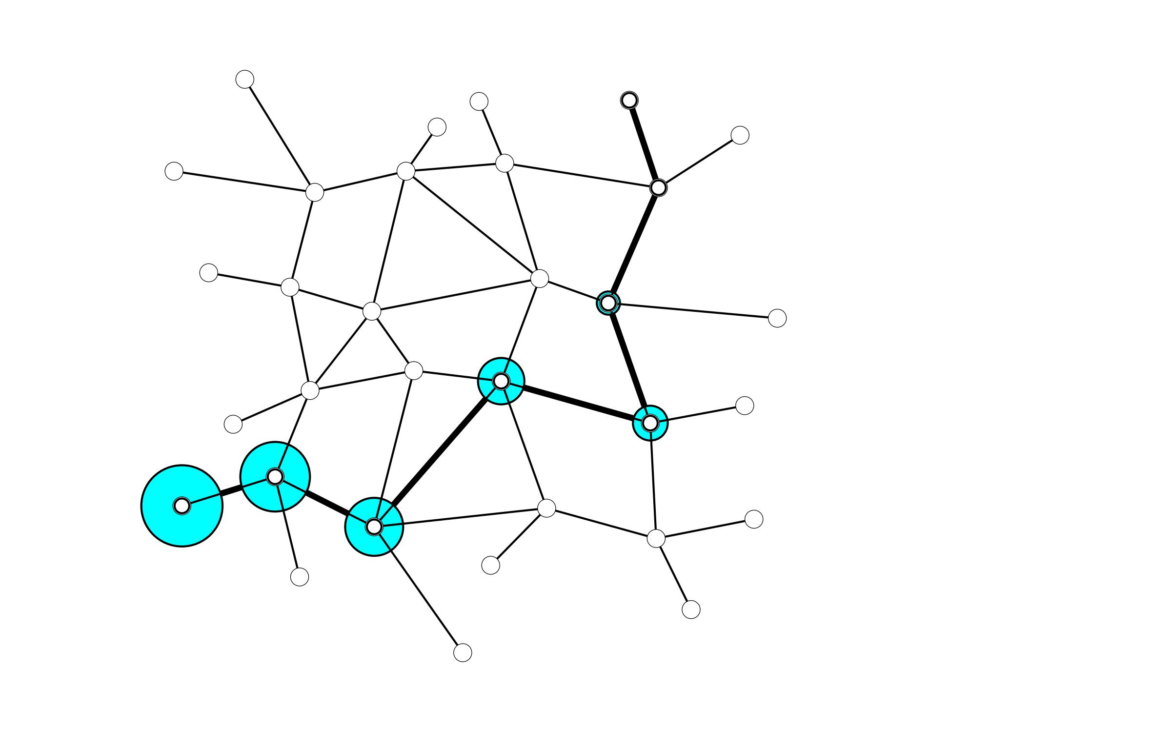
network = Network.from_obj(compas.get('grid_irregular.obj'))

start, end = random.sample(network.leaves(), 2)
path = network.shortest_path(start, end)
points = network.nodes_attributes('xy', keys=path)

polyline = Polyline(points)
circles = [Circle([point, [0, 0, 1]], 0.1 * index) for index, point in enumerate(points)]

plotter = Plotter()

plotter.add(network)
plotter.add(polyline, linewidth=3)
plotter.add_from_list(circles, facecolor=(0, 1, 1))

plotter.zoom_extents()
plotter.show()

Basic Usage

Using compas_plotters.Plotter is very simple.

Create a plotter instance.
Add Objects.
Optionally zoom the extents of all objects that were added.
Show the plot.

plotter = Plotter()

# add objects

plotter.zoom_extents()
plotter.show()

COMPAS geometry objects and data structures can be added using compas_plotters.Plotter.add(). By adding an object, a corresponding “artist” is created automatically in the background, and the plotter will use the artist to visualize the object.

The artists provide many configuration options to modify the display styles of the objects. The compas_plotters.Plotter.add() method accepts additional keyword arguments corresponding to those configuration options. See the API reference of the individual artists for the available options per object type.

point = Point(0, 0, 0)

plotter.add(point, size=10, facecolor=(1.0, 0.7, 0.7), edgecolor=(1.0, 0, 0))

Alternatively, multiple objects of the same type can also be added using compas_plotters.Plotter.add_from_list(). In this case all configurations options will be applied uniformly to all objects in the list.

cloud = Pointcloud.from_bounds(10, 10, 0, 100)

plotter.add_from_list(cloud.points, size=1, facecolor=(1.0, 0.7, 0.7), edgecolor=(1.0, 0, 0))

Geometry Objects

Most of the geometry primitives are supported and can be added to a plotter instance as described above:

Bezier curves and pointclouds are currently not available yet, but will be added as well. Note that in all cases, the z coordinates of the objects are simply ignored, and only a 2D representation is depicted.

plotter.add(point)
plotter.add(vector)
plotter.add(line)
plotter.add(circle)
plotter.add(ellipse)
plotter.add(polyline)
plotter.add(polygon)

Data Structures

Of the three types of data structures, only network and mesh are supported. Also in this case, the z coordinates of the geometry is ignored, and only a 2D representation is depicted.

plotter.add(point)
plotter.add(vector)

Visualisation Options

Line and Polyline

Name	Value	Default
`linewidth`	`float`	`1.0`
`linestyle`	`{'solid', 'dotted', 'dashed', 'dashdot'}`	`'solid'`
`color`	`tuple`	`(0.0, 0.0, 0.0)`
`draw_points`	`bool`	`False`

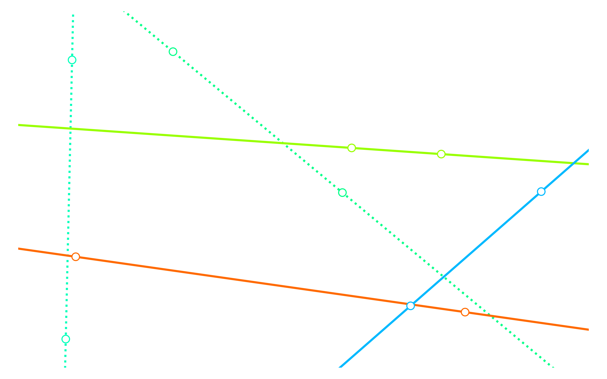
pointcloud = Pointcloud.from_bounds(8, 5, 0, 10)

for a, b in grouper(pointcloud, 2):
    line = Line(a, b)
    plotter.add(line,
                linewidth=2.0,
                linestyle=random.choice(['dotted', 'dashed', 'solid']),
                color=i_to_rgb(random.random(), normalize=True),
                draw_points=True)

Circle, Ellipse, Polygon

Name	Value	Default
`linewidth`	`float`	`1.0`
`linestyle`	`{'solid', 'dotted', 'dashed', 'dashdot'}`	`'solid'`
`facecolor`	`tuple`	`(1.0, 1.0, 1.0)`
`edgecolor`	`tuple`	`(0.0, 0.0, 0.0)`
`alpha`	`float`	`1.0`
`fill`	`bool`	`True`

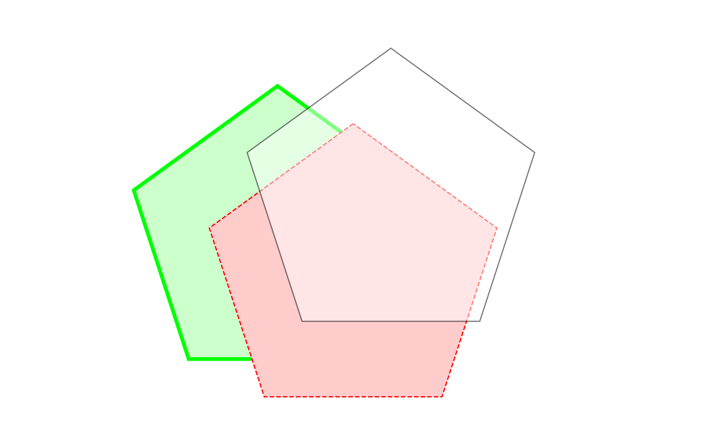
poly1 = Polygon.from_sides_and_radius_xy(5, 1.0)
poly2 = Polygon.from_sides_and_radius_xy(5, 1.0).transformed(Translation.from_vector([0.5, -0.25, 0]))
poly3 = Polygon.from_sides_and_radius_xy(5, 1.0).transformed(Translation.from_vector([0.75, +0.25, 0]))

plotter.add(poly1, linewidth=3.0, facecolor=(0.8, 1.0, 0.8), edgecolor=(0.0, 1.0, 0.0))
plotter.add(poly2, linestyle='dashed', facecolor=(1.0, 0.8, 0.8), edgecolor=(1.0, 0.0, 0.0))
plotter.add(poly3, alpha=0.5)

Points

Name	Value	Default
`size`	`int`	`5`
`facecolor`	`tuple`	`(1.0, 1.0, 1.0)`
`edgecolor`	`tuple`	`(0.0, 0.0, 0.0)`

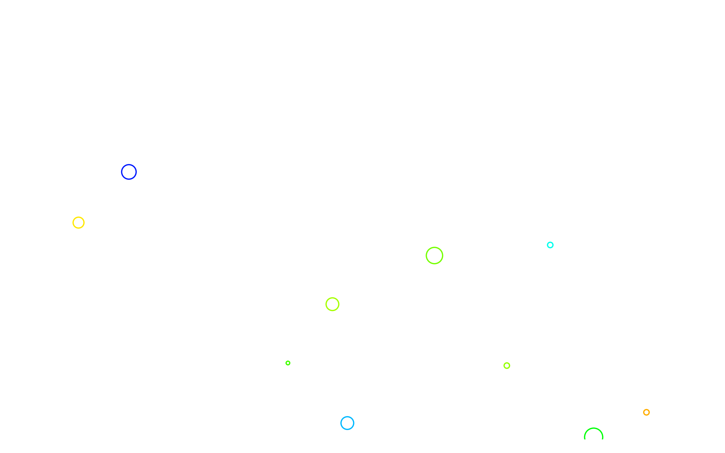
pointcloud = Pointcloud.from_bounds(8, 5, 0, 10)

for point in pointcloud:
    plotter.add(point, size=random.randint(1, 10), edgecolor=i_to_rgb(random.random(), normalize=True))

Vectors

Name	Value	Default
`point`	`compas.geometry.Point`	`None`
`draw_point`	`bool`	`False`
`color`	`tuple`	`(0.0, 0.0, 0.0)`

pointcloud = Pointcloud.from_bounds(8, 5, 0, 10)

for index, (a, b) in enumerate(pairwise(pointcloud)):
    vector = b - a
    vector.unitize()
    plotter.add(vector, point=a, draw_point=True, color=i_to_red(max(index / 10, 0.1), normalize=True))

Dynamic Plots

Dynamic plots, or animations, can be made with the “on” decorator compas_plotters.Plotter.on(). Simply add the decorator to a callback functions that updates the geometry in the plot at a specified interval.

@plotter.on(interval=0.1, frames=50)
def move(frame):
    for a, b in pairwise(pointcloud):
        vector = b - a
        a.transform(Translation.from_vector(vector * 0.1))

For example, the following will update the locations of the points of a pointcloud for 50 frames and with an interval of 0.1 seconds between the frames.

from compas.geometry import Pointcloud, Translation
from compas.utilities import i_to_red, pairwise

from compas_plotters import Plotter

plotter = Plotter(figsize=(8, 5))

pointcloud = Pointcloud.from_bounds(8, 5, 0, 10)

for index, (a, b) in enumerate(pairwise(pointcloud)):
    artist = plotter.add(a, edgecolor=i_to_red(max(index / 10, 0.1), normalize=True))

plotter.add(b, size=10, edgecolor=(1, 0, 0))
plotter.zoom_extents()
plotter.pause(1.0)

@plotter.on(interval=0.1, frames=50)
def move(frame):
    for a, b in pairwise(pointcloud):
        vector = b - a
        a.transform(Translation.from_vector(vector * 0.1))

If you want to keep the plot alive at the end of the animation, add a call to show.

plotter.show()

To save the animation to an animated gif, set the record flag to True, and add a recording path.

@plotter.on(interval=0.1, frames=50, record=True, recording='docs/_images/tutorial/plotters_dynamic.gif')
def move(frame):
    for a, b in pairwise(pointcloud):
        vector = b - a
        a.transform(Translation.from_vector(vector * 0.1))

Interactive Plots

Coming soon.