Elements
This page shows how different types of Element objects are added and edited with the Structure object, here the example Structure object is given as mdl. The Element objects represent linear, surface and solid finite elements connecting different nodes of the structure.
Adding elements
Element objects are added to the Structure object with the .add_element() and .add_elements() methods, by giving the list(s) of nodes that the element(s) connect to, as well as the element type as a string. If a single element is being added with .add_element(), then the node numbers are given in nodes, while if multiple elements are added with .add_elements(), lists of nodes are given through elements. The Element objects are added to the .elements dictionary of the Structure, from the classes found in module compas_fea.structure.element, where the class names match the string entered for the element type type.
The element types include, amongst others, 1D elements: SpringElement, BeamElement, TrussElement, 2D elements: ShellElement, MembraneElement, and 3D elements: PentahedronElement, TetrahedronElement, HexahedronElement. Note: to date, not all elements types are consistently available across all FE solvers, Abaqus, OpenSees and Ansys.
As with nodes, the elements will be added with integer keys numbered sequentially starting from 0. Note: currently no more than one element can exist for the same collection of nodes, i.e. no overlapping elements are allowed. If you use .add_element() and an element already exists, nothing else will be added.
mdl.add_element(nodes=[0, 1, 4], type='ShellElement')  # a single element added

mdl.add_elements(elements=[[0, 4], [1, 4], [2, 4], [3, 4]], type='BeamElement')  # multiple elements added
For Abaqus, adding elements will also create a set for each individual element. So for example, when element 4 is written to the input file, an element set named element_4 (corresponding to element number 5 in Abaqus) will also be created. The utility of this is that individual elements can be referenced to whenever needed, which is useful for selectively assigning a thickness, material, section or orientation to specific elements by way of their number (see some of the examples for demonstrations of this).
Viewing elements
The Element objects that have been added to the Structure can be viewed through their integer key and the attributes .__name__, .axes, .nodes, .number, element_property and .thermal (the thermal boolean attribute is a placeholder for later functionality). A summary of the element can be viewed by printing the element to the terminal.
 >>> mdl.elements[3]  # element number 3
 BeamElement(3)

 >>> print(mdl.elements[3])  # print a summary of element 3

 compas_fea BeamElement object
 -----------------------------
 nodes      : [3, 4]
 number     : 3
 thermal    : False
 axes       : {'ex': [1, 0, 0]}
 element_property : ep_circ

 >>> mdl.elements[3].nodes  # nodes that element 3 connects
 [3, 4]

 >>> mdl.elements[3].__name__  # type of element
'BeamElement'

 >>> mdl.elements[3].thermal  # thermal boolean
 False
Element index
A geometric key to integer key index dictionary is accessed through .element_index, where the geometric key is taken as the element centroid and the key is the number of the element. The .element_index dictionary is similar in function to the .node_index dictionary, and is useful for checking if an element exists (see methods below).
>>> mdl.element_index  # view the structure element_index
{'-2.500,-2.500,2.500': 0, '2.500,-2.500,2.500': 1, '2.500,2.500,2.500': 2, '-2.500,2.500,2.500':  3}
Methods
It can be checked if an element is already present in the Structure object (via .element_index in the background), by a query with the method .check_element_exists(). This method must be given the list of nodes the element would be connected to, or the location xyz of where its centroid would be. As the check is based on the centroid of the element, it does not matter the order that the nodes are given in the list nodes. If an element exists, the method will return the integer key, if not, None will be returned.
>>> mdl.check_element_exists(nodes=[1, 4])  # does an element exist connecting nodes 1 and 4
1

>>> mdl.check_element_exists(nodes=[1, 2, 3])  # does an element exist connecting nodes 1, 2 and 3
None

>>> mdl.check_element_exists(xyz=[0, 10, 5])  # does an element exist with centroid at [0, 10, 5]
3
The number of elements in the Structure can be returned with the method .element_count(), which essentially takes the length of the dictionary keys in structure.elements.
>>> mdl.element_count()  # return the total number of elements in structure.elements
5
An element centroid can be determined by the method .element_centroid().
>>> mdl.element_centroid(element=3)  # return the centroid of element number 3
(-2.5, 2.5, 2.5)
Axes
Giving a dictionary for the argument axes when adding the element, will store {'ex': [], 'ey': [], 'ez': []} in the Element object’s .axes attribute. The 'ex', 'ey' and 'ez' lists are the element’s local x, y and z axes, and are used for example when orientating cross-sections, using anisotropic materials, or for aligning rebar in concrete shells. If no axes data are given, it is left up to the finite element solver to determine default local axes values. This default alignment, if supported by the software, is often based on the global axes of the model, thus it is important to understand if these defaults are suitable, especially for an element geometry that does not align well with the global x, y, z directions. If for example you create a BeamElement for Abaqus that is perfectly vertical, you will get an error from Abaqus that it was not able to work out a local orientation, as it tries to align beam elements to the global x and y directions. OpenSees demands explicitly a local orientation for beams, so this step of defining the local axes cannot be skipped.
For the local axes of a line element such as a beam, the 'ex' axis represents the cross-section’s major axis, 'ey' is the cross-section’s minor axis, and 'ez' is the axis along the element. For surface elements, the 'ex' and 'ey' axes represent the in-plane local axes, with 'ez' then representing the positive normal vector. The CAD functions (described in the CAD topic) that add elements to the Structure from geometry in the workspace, will automate some of these axis definitions/tasks, so see the Rhino and Blender pages later on how the CAD environment can help prescribe these orientations more effectively.
mdl.add_element(nodes=[1, 3], type='BeamElement', axes={'ex': [0, -1, 0]}) # add a beam with its major axis ex
mdl.add_element(nodes=[0, 1, 4], type='ShellElement', axes={'ex': [1, 1, 0], 'ey': [-1, 1, 0], 'ez': [0, 0, 1]})
Elements
1D elements
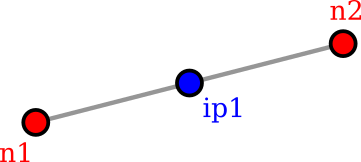
One dimensional elements such as truss (TrussElement) and beam (BeamElement) elements are currently first order linear elements defined by two nodes, which are the start (n1) and end (n2) points of a straight line. An internal node is currently not supported for second order parabolic elements. For the modelling of a curved shaped beam, use many straight segments. The single integration point (ip1) is at the midpoint of the line element.
2D elements
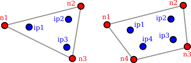
Two dimensional elements such as membrane (MembraneElement) and shell (ShellElement) elements are currently first order linear defined by either three (n1, n2, n3) or four (n1, n2, n3, n4) nodes. These nodes are the corners of straight-sided elements, intermediate edge nodes are currently not supported for second order parabolic elements. For modelling a curved edge, use many straight segments. There are three or four internal integration points within the element (ip1 through to ip3 or ip4).
3D elements
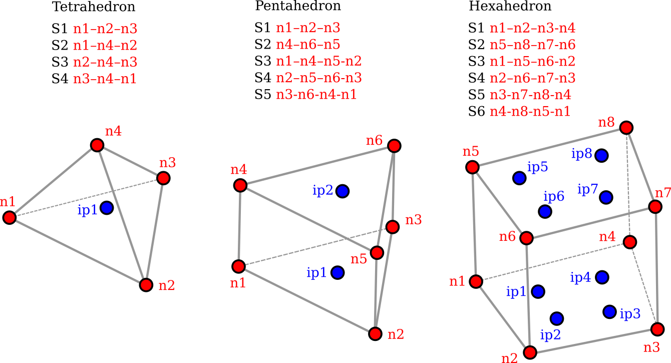
Three dimensional solid elements are also currently first order (linear), they are defined by four nodes (TetrahedronElement with four sides S1 to S4), six nodes (PentahedronElement with five sides S1 to S5) or eight nodes (HexahedronElement with six sides S1 to S6). The nodes are the corners of flat-faced elements and should be added in the order shown below. Intermediate edge nodes are currently not supported for second order parabolic elements. For a curved edge/face, use many straight segments/faces for modelling. There is one internal integration point for a TetrahedronElement (ip1). two for a PentahedronElement (ip1 and ip2) and eight for a HexahedronElement (ip1 to ip8).
Meshing
The compas_fea package supports the use of Triangle and TetGen via the Python wrapper MeshPy, and is independent of any CAD environment. MeshPy can easily be installed via pip on Linux systems, while a .whl file is recommended for Windows from the excellent resource page here .
2D elements
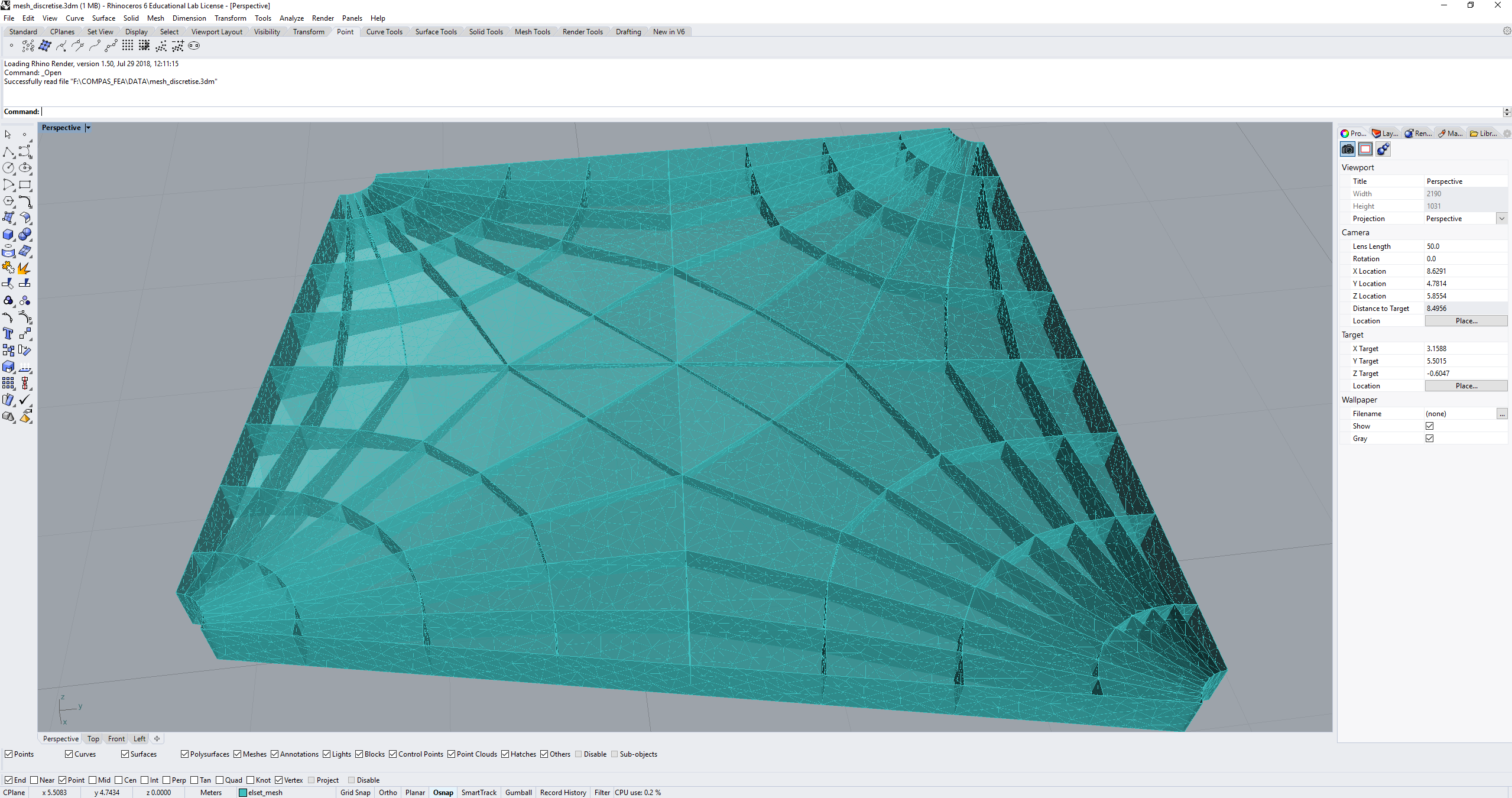
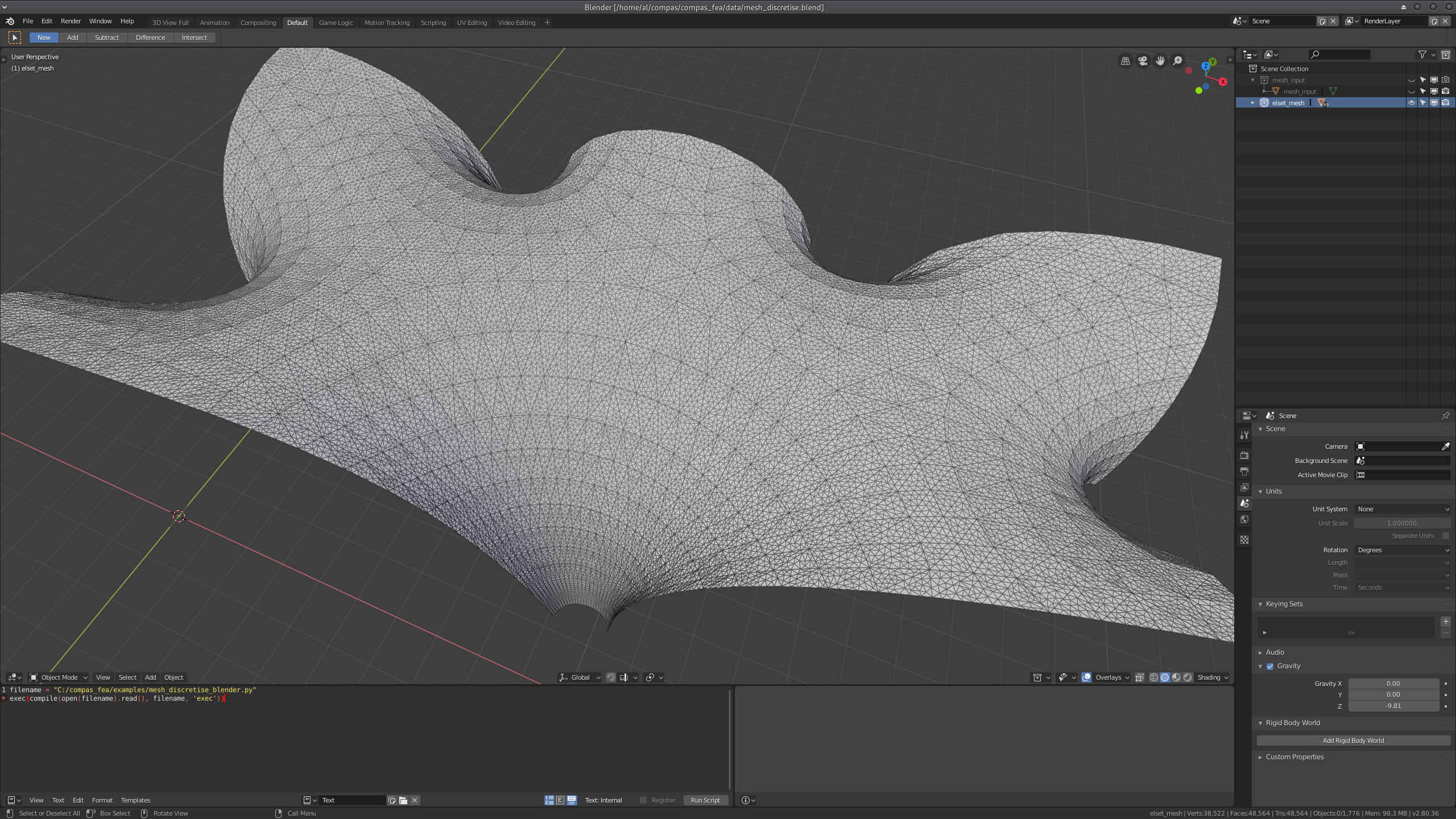
There are two main ways to discretise coarse meshes into denser forms for an accurate finite element analysis. The first is to use the discretisation and subdivision methods in the core compas package, namely those under compas.topology. The second is to use the discretise_faces() function found in compas_fea.utilities.meshing. This takes the vertices and faces of the coarse mesh, a target triangle element size, and a minimum angle min_angle for the triangles’ internal angles. The function will then discretise the coarse mesh with MeshPy (via Triangle) and return a finer mesh for each of the faces of the input mesh. The returned discretised faces will not be welded together to form a single mesh (this is also not needed when adding elements to the Structure object anyway).
The function call compas_fea.utilities.meshing.discretise_faces has been conveniently wrapped for use in Rhino and Blender with the functions rhino.discretise_mesh and blender.discretise_mesh. Which requires: 1) the structure to add the discretised mesh to, 2) the guid or object of the triangulated coarse mesh in the workspace, 3) the layer to plot the finer mesh to, and 4) the required target and min_angle parameters for the final triangles. These functions will automatically sort out the vertices and faces arguments needed in discretise_faces() by extracting them from the mesh geometry. A call using these functions may look like the following, which gives example meshing results afterwards for Rhino and Blender.
from compas_fea.cad import rhino
from compas_fea.structure import Structure

import rhinoscriptsyntax as rs

mdl = Structure(name='mesh_discretise', path='C:/Temp/')  # make an empty/base structure

guid = rs.ObjectsByLayer('mesh_input')[0]  # grab the coarse mesh from the workspace
rhino.discretise_mesh(mdl, mesh=guid, layer='elset_mesh', target=0.050, min_angle=15)  # discretise
3D elements
When discretising a solid volume into finite elements, the first step is usually to create a mesh that represents the outer-surface of the solid. This mesh can be represented as a triangulated mesh with somewhat equally sized triangles, as there are many algorithms for creating tetrahedron elements from an outer surface by adding them across the internal volume. A function has been set-up to facilitate converting a collection of triangles and vertices data representing the outer-surface, into tetrahedron elements. This is the function tets_from_vertices_faces(), found in compas_fea.utilities.meshing, where the vertices co-ordinates, the triangle faces, and a volume constraint (optional) are given. The outputs of using the function are the points and indices of the tetrahedron corners.
If you are in a CAD environment, you can use the geometry from a constructed triangulated outer-surface mesh to create and automatically add tetrahedron elements to your Structure object. In Rhino, use .add_tets_from_mesh() from compas_fea.cad.rhino, and in Blender, use the same name of function .add_tets_from_mesh() from compas_fea.cad.blender. These functions effectively wrap around tets_from_vertices_faces() and add the elements to the Structure object for you. These function calls could look like:
from compas_fea.cad import rhino

import rhinoscriptsyntax as rs

mesh = rs.ObjectsByLayer('mesh')[0]  # grab the mesh from layer 'mesh'

rhino.add_tets_from_mesh(structure=mdl, name='elset_tets', mesh=mesh,
                         draw_tets=True, layer='tets', volume=0.1)  # make and add tets
from compas_fea.cad import blender

from compas_blender.utilities import get_objects

mesh = get_objects(name='mesh')  # grab the mesh with name 'mesh'

blender.add_tets_from_bmesh(structure=mdl, name='elset_tets', bmesh=mesh,
                            draw_tets=False, volume=0.002)  # make and add tets
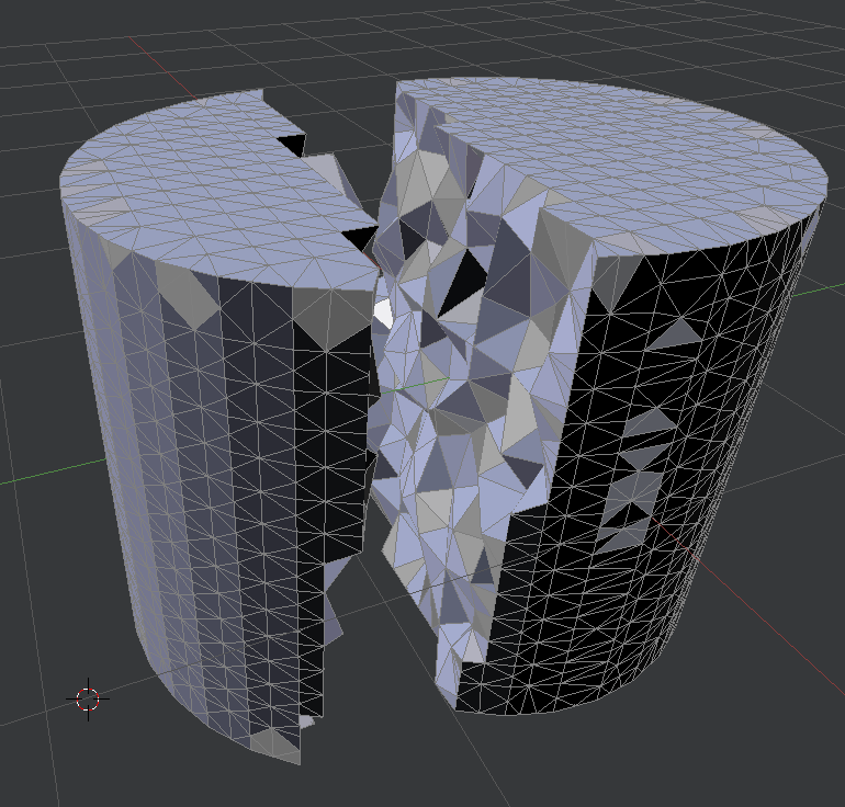
For both the Rhino and Blender cases the following must be given: 1) the Structure object structure to add the tets to, 2) the name of the element set to make after adding the tetrahedrons, 3) whether to draw mesh representations of the tetrahedrons with the boolean draw_tets (they will be drawn on layer layer), and 4) the volume constraint if desired with volume. For the Rhino case above, a mesh was gathered from layer 'mesh', and for Blender the mesh named mesh. The tetrahedrons will have been added to structure.elements and the created element set stored under structure.sets. Note: take care when plotting a dense collection of tetrahedrons with draw_tets=True, as it can easily overload the viewport with many individual meshes. An example of some generated and plotted tetrahedrons is shown below, stemming from the outer surface mesh of a cylinder.