Materials

Elastic

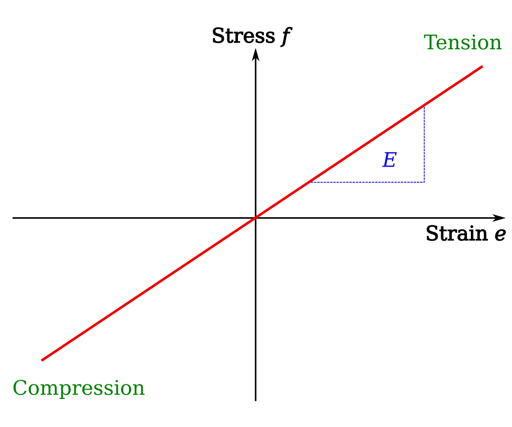
The simplest material model is the elastic, isotropic and homogeneous material ElasticIsotropic. This takes the Young’s modulus E [Pa], Poisson’s ratio v and density p [kg per cubic metre]. Additionally, it can be stated if the material should allow tension or compression, given as boolean arguments and defaulting to True.

from compas_fea.structure import ElasticIsotropic

mdl.add(ElasticIsotropic(name='mat_elastic', E=10**10, v=0.3, p=1500, tension=True, compression=True))

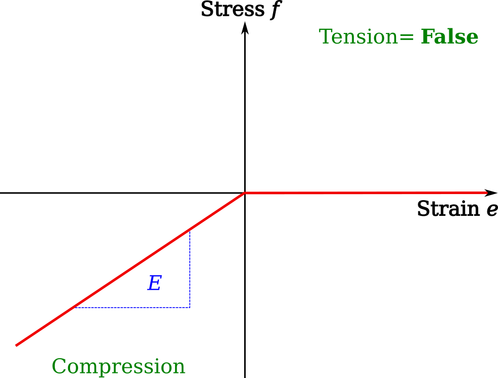
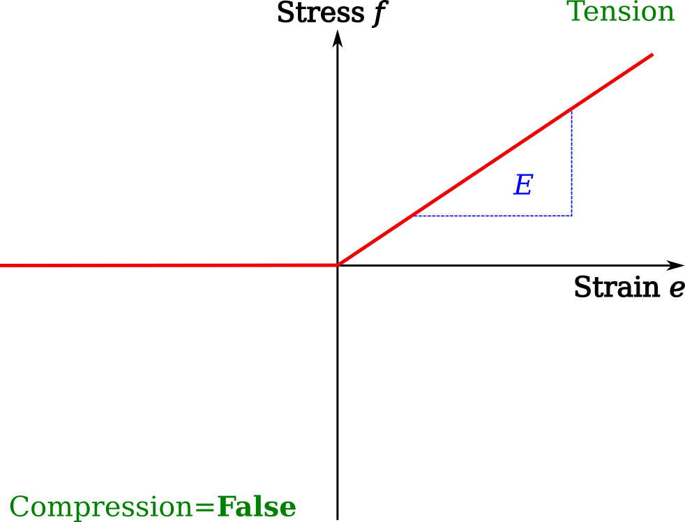
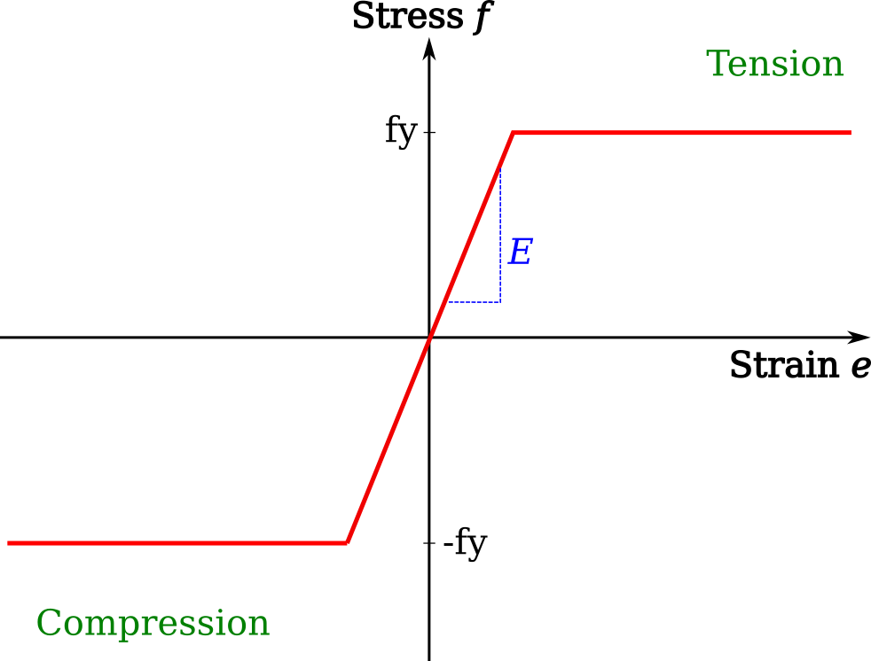
The standard elastic material model is shown below, where tension is taken as positive. To allow only compression, set tension=False and to allow only tension, set compression=False.

Stiff

A very stiff linear elastic material can be made by creating a Stiff object. This material is essentially identical to ElasticIsotropic but with E taken as very high, v as 0.3 and p as 0.1, and is more of a modelling aid than a real structural material.

from compas_fea.structure import Stiff

mdl.add(Stiff(name='mat_stiff'))

Elastic–plastic

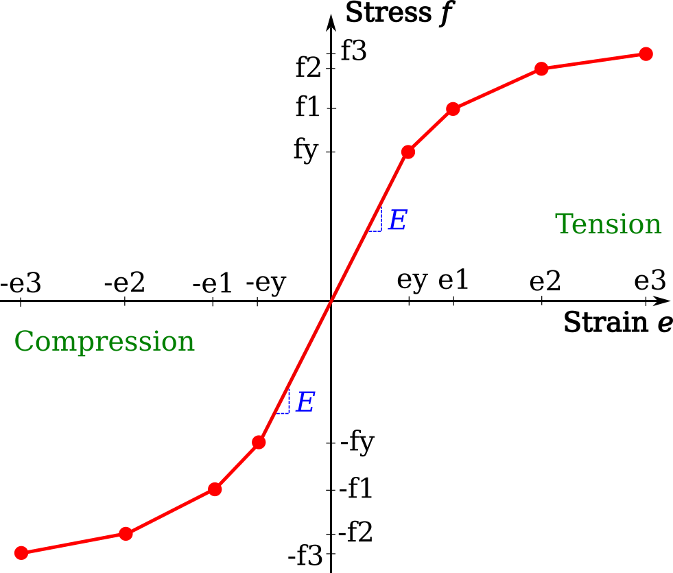
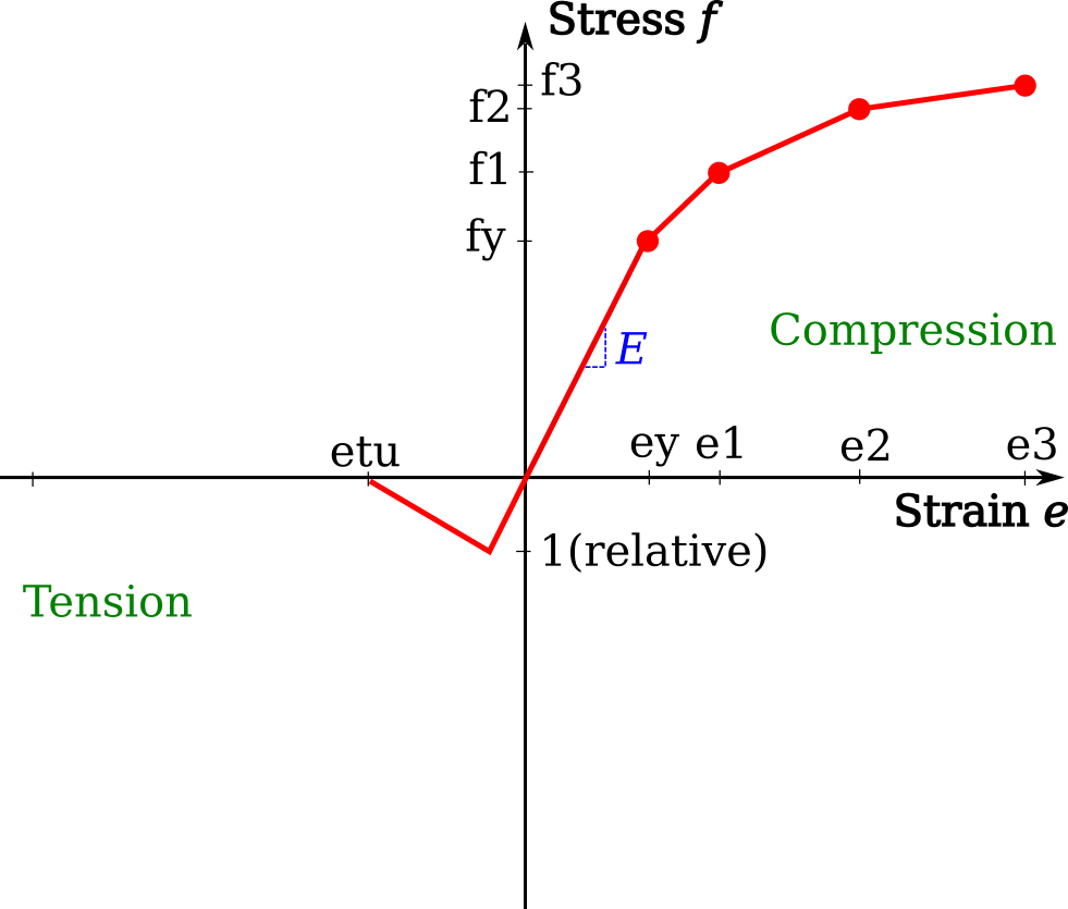
The ElasticPlastic class can be used to make a general isotropic and homogeneous non-linear material object, with the same shape of stress–strain curve in both compression and tension. The elastic input data is the same as with the ElasticIsotropic class, given by Young’s modulus E [Pa], Poisson’s ratio v and density p [kg per cubic metre]. For the plastic description of the material, use lists of plastic stresses f [Pa] and plastic strains e [total strain minus yield strain]. The first value of f should be the stress at the end of the elastic region, i.e. the yield stress, and the first value of e should be zero, i.e. the beginning of plastic straining. Continue to give pairs of plastic stress and plastic strain to define the complete behaviour. To add the general elastic–plastic stress–strain data curve below as data to the ElasticIsotropic class, the input (with variables representing numbers) would look like:

from compas_fea.structure import ElasticPlastic

f = [fy, f1, f2, f3]
e = [0, e1 - ey, e2 - ey, e3 - ey]

mdl.add(ElasticPlastic(name='mat_plastic', E=E, v=v, p=p, f=f, e=e))

Steel

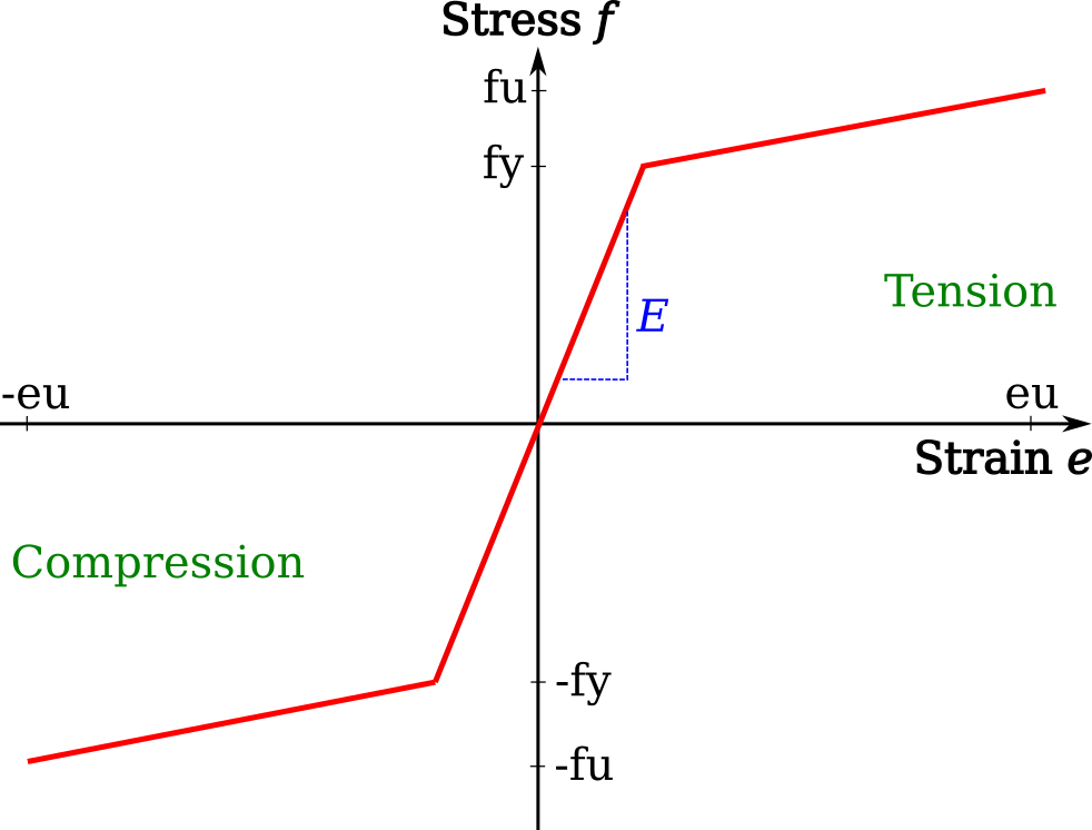
The Steel class will create an object based on structural steel, so it can be added it to the Structure. The string name for the material is given, while the yield stress fy [MPa], Young’s modulus E [GPa], Poisson’s ratio v and density p [kg per cubic metre], will all default to common values used in design if no user specific values are given. The type of linear material behaviour after first yield can be defined through the ultimate stress and strain fu [Pa] and eu [%]. Note: that the yield stress is given in units of [MPa] and Young’s modulus in [GPa], but then stored, as with all materials, as [Pa]. By default, an elastic-plastic type of behaviour will be made with fy equal to fu.

from compas_fea.structure import Steel

mdl.add(Steel(name='mat_steel', fy=355, E=210, v=0.3, p=7850))

from compas_fea.structure import Steel

mdl.add(Steel(name='mat_steel', fy=355, fu=500, E=210, eu=10))

Concrete

There are currently three material models for concrete, a Eurocode 2 model Concrete, a smeared crack model ConcreteSmearedCrack, and a damaged plasticity model ConcreteDamagedPlasticity. The key features of these three models are described below:

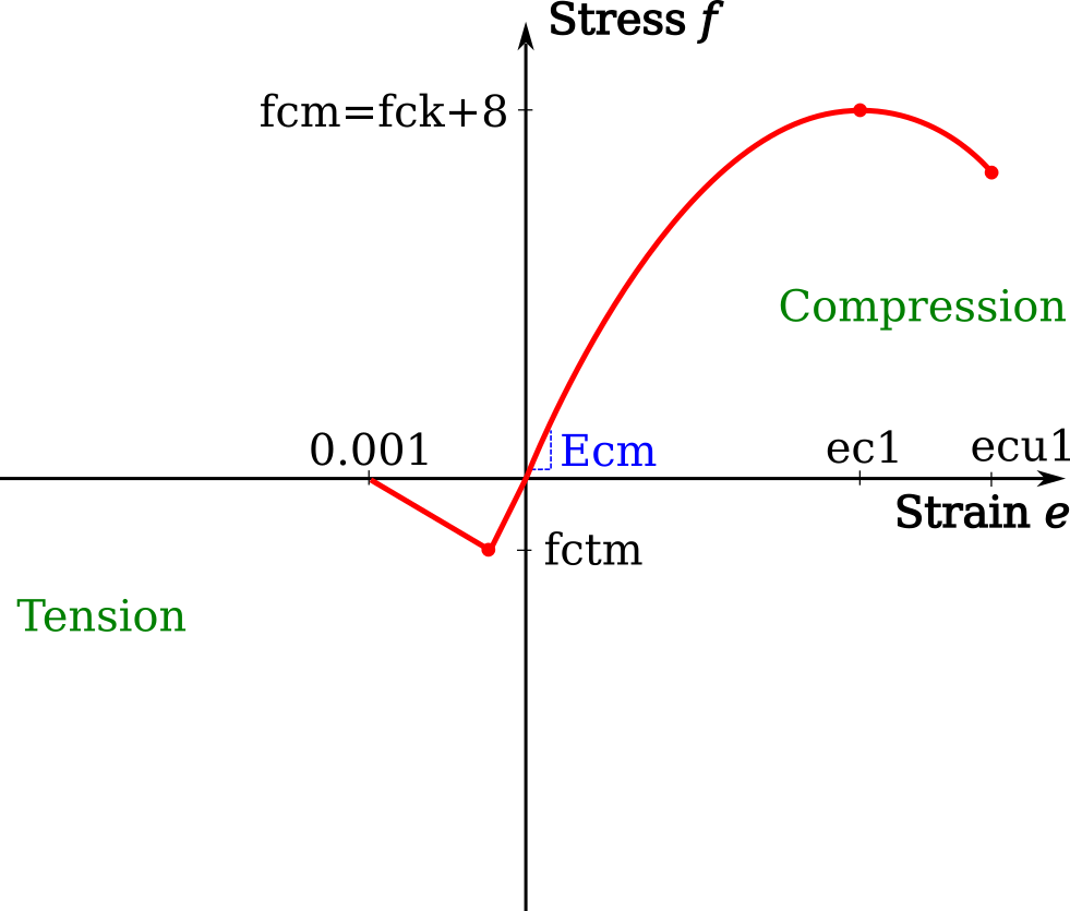
• The easiest concrete material object to create is with the Concrete class, which requires mainly the characteristic (5%) 28 day cylinder strength in MPa (up to 90 MPa). Default values of the Poisson’s ratio v=0.2 and density p=2400 are taken unless specified otherwise. As per Eurocode 2 Part 1-1 (particularly Table 3.1), key material data is derived from knowing the characteristic cylinder strength fck. The Concrete model includes: 1) the compressive stress–strain model of Eurocode 2 Part 1-1 Clause 3.1.5, 2) the mean Young’s modulus, tensile and compressive stresses from Eurocode 2 Part 1-1 Table 3.1, and 3) will assume a linear elastic response until the tensile cracking stress, followed by a drop to zero tensile stress at 0.1 % strain.

from compas_fea.structure import Concrete

mdl.add(Concrete(name='mat_concrete', fck=90, v=0.2, p=2400))

• The ConcreteSmearedCrack class (based on the Abaqus smeared crack material) creates a general concrete material model object. The Young’s modulus E [Pa], Poisson’s ratio v and density p are all explicitly given, as no defaults are assumed. The compressive stress–strain data are given with plastic stresses fc [Pa] (positive) and plastic strains ec in exactly the same way as the ElasticPlastic model. The first value of fc is the stress at the end of the elastic region defined by slope E, paired with the first value of ec of zero. For the tensile stresses, tension stiffening uses ft and et, where ft are not the absolute values of tensile stress, but the relative tensile stress from the point of cracking. So the first data pairs are ft as 1 at et of 0, then dropping to ft as 0 at another value of et (0.001 recommended). Before cracking, the tensile stress–strain behaviour is linear, using the same Young’s modulus E as for compression. Finally, the failure ratios fr are given, which are the ratio of the ultimate bi-axial to uni-axial compressive ultimate stress (default 1.16) and the ratio of uni-axial tensile to compressive stress at failure (default 0.0836), the latter will give a tensile failure stress of 35 * 0.0836 = 2.926 if the concrete maximum compressive stress is 35 MPa. To add the general concrete stress–strain data curve below as data to the ConcreteSmearedCrack class, the input (with variables representing numbers, and the cracking stress as 10% of peak stress f3) would look like:

from compas_fea.structure import ConcreteSmearedCrack

fc = [fy, f1, f2, f3]
ec = [0, e1 - ey, e2 - ey, e3 - ey]
ft = [1, 0]
et = [0, etu]
fr = [1.16, 0.10]

mdl.add(ConcreteSmearedCrack(name='mat_concrete', E, v, p, fc, ec, ft, et, fr))

• The ConcreteDamagedPlasticity material model is used for concrete and other quasi-brittle materials (and is based here and quoted from the Abaqus damaged plasticity material). The class takes the Young’s modulus E, Poisson’s ratio v and density p as no defaults are assumed, as well as lists damage, hardening and stiffening. For damage, a list is given of: the dilation angle in degrees, flow potential eccentricity, the ratio of initial equibiaxial to uni-axial compressive yield stress, the ratio of the second stress invariant on the tensile meridian to that on the compressive meridian, and the viscosity parameter. For the input hardening, a list is given of: the compressive yield stress, inelastic crushing strain, inelastic crushing strain rate, and temperature. Finally, for stiffening, a list of: remaining direct stress after cracking, direct cracking strain, direct cracking strain rate, and temperature.

Timber

Timber models are to be developed.